Barbados Stock Exchange
 Image credit: Unsplash
Introduction
I have a vested interest in finding interesting datasets related to Barbados as that’s where I’m from.
One site which caught my interest is the Barbados Stock Exchange.
Now I’m currently ignorant when it comes to all things stocks, but I do see they offer on their website the ability to download monthly reports, and I do understand ‘free to download’.
Downloading Files
The first thing we need to do is load the information into our tool of choice, yet they’re quite a few files we’d need to download and edit.
Here we can take advantage of some automation to help us out, my tool of choice for this will be R.
We’ll first load our libraries and start writing our code.
library(conflicted)
library(tidyverse)
conflict_prefer("filter", "dplyr")

library(clock)
library(gt)
Prep Work
First we download and look at some of the files manually. We thus confirm that we can download the reports as csv files from the link, > [Domain]/reports/monthly/download-csv?tradeDate=[Date] > >where [Date] is the the date of interest in the format of yyyy-mm-dd.
We can generate a sequence of dates using seq and clock which we can paste unto our base link.
This will give us a list of links for all the files we’re interested in.
# Download the data from the base link
base_link <- "https://bse.com.bb/reports/monthly/download-csv?tradeDate="

# Specify dates of interest
from <- clock::year_month_day(1910, 1)
to <- clock::year_month_day(2022, 1)

# Generate download links
download_links <- tibble::tibble(
  link = paste0(base_link,
                seq(from, to, by = 1),
                "-01")
)
We can confirm that the links were created as expected by looking at a few with the following code.
# Show some of our generated links
download_links %>%
  head() %>%
  gt::gt(rowname_col = NULL) %>%
  gt::tab_header(
    title = "List of generated links"
)| List of generated links |
|---|
| link |
| https://bse.com.bb/reports/monthly/download-csv?tradeDate=1910-01-01 |
| https://bse.com.bb/reports/monthly/download-csv?tradeDate=1910-02-01 |
| https://bse.com.bb/reports/monthly/download-csv?tradeDate=1910-03-01 |
| https://bse.com.bb/reports/monthly/download-csv?tradeDate=1910-04-01 |
| https://bse.com.bb/reports/monthly/download-csv?tradeDate=1910-05-01 |
| https://bse.com.bb/reports/monthly/download-csv?tradeDate=1910-06-01 |
Downloading Files
In our prep work, we created 1345 links to now download our files. That’s a bit, but thankfully we’re not doing this by hand, instead we’ll also be leveraging R here as well.
We’ll first create a folder called “Stock_Files” to store our downloaded files to, as I may rerun this script multiple times, I’ll only download the files if this folder doesn’t exist.
We’re also not particularly interested in any one file, so we’ll just assign them temporary names.
# Note how many files we're interested in
val <- nrow(download_links)

# If I've downloaded the files already, just use them, otherwise download them
if( length( list.dirs(path = "./Stock_Files") ) >= 1 ) {
  stock_dir <- paste0(getwd(),"/Stock_Files")
  stock_files <- list.files(path = stock_dir,
                           pattern = "csv$")

} else {

  # Create a directory
  dir.create("./Stock_Files",
             showWarnings = TRUE,
             recursive = FALSE,
             mode = "0777")

  # Create multiple temporary file names
  stock_files <- tibble::tibble(
    id = seq(1, val, 1),
    file_path = seq(1, val, 1) %>%
      map(~ tempfile(
        pattern = paste0("temp_stock_",.x),
        tmpdir = stock_dir,
        fileext = ".csv"))
  )

  # Download the files using temporary directory and file names
  for(i in seq_along(1:val)){
    try(
      download.file(download_links$link[i],
                    stock_files$file_path[[i]],
                    method = "wininet"),
      silent = TRUE)
  }

}
We’ve successfully downloaded our files, but when we open some of them, we notice they’re empty!
It turns out only some of the files have information, those without information, are simply blank.
Interestingly, if we examine some of the empty files, we notice they’re only 3 bytes. We can use this to our advantage by deleting any file which has a size of 3 bytes or less.
# Record details on the files downloaded
detail_files <- fileSnapshot(stock_dir)


# Some months and thus files did not have any information, we make a list of those files
delete_files <- detail_files$info %>%
  select(size) %>%
  mutate(file = row.names(.),
         file = paste0(stock_dir,"/",file)) %>%
  filter(size <= 3 & str_detect(file, "csv$"))

# Delete all the unwanted files
invisible(
  sapply(delete_files$file, unlink)
)


## Read in the remaining files

# Note files which are kept
kept_files <- detail_files$info %>%
  select(size) %>%
  mutate(file = row.names(.),
         file = paste0(stock_dir,"/",file)) %>%
  filter(size > 3 & str_detect(file, "csv$"))
Now after this, we can at last read our kept files into memory.
# read in all the CSV files
data_raw <- map_dfr(.x = kept_files$file,
                    .f = read_csv,
                    skip = 1,
                    col_types = cols(
                      `Trade Date` = col_character(),
                      Security = col_character(),
                      Volume = col_character(),
                      High = col_character(),
                      Low = col_character(),
                      `Last Close` = col_character(),
                      `Current Close` = col_character(),
                      `Price Change` = col_character(),
                      `Bid Price` = col_character(),
                      `Ask Price` = col_character()
                    ))
Of the 1345 files downloaded, we deleted 0 and kept only 73.
Why so little? Well it so happens that the Stock Exchange only start recording information from around 2015, and we started our count from 1910, quite inefficient of us.
Well the reason we did this (notice I’m still using we), was to show how we can find ways to remove unneeded files without much issue. (That, and I was too lazy to manually check when useful information was recorded.)
Table showing Raw Data
# Show the first few values of the files we downloaded
data_raw %>%
  head() %>%
gt::gt()| Trade Date | Security | Volume | High | Low | Last Close | Current Close | Price Change | Bid Price | Ask Price |
|---|---|---|---|---|---|---|---|---|---|
| 2015-01-01 | ABV | 1,500 | 0.32 | 0.32 | 0.00 | 0.32 | 0.00 | 0.25 | 0.30 |
| 2015-01-01 | BHL | 2,144 | 2.90 | 2.90 | 0.00 | 2.90 | 0.00 | 2.50 | 2.88 |
| 2015-01-01 | BCO | 13,899 | 1.90 | 1.65 | 0.00 | 1.82 | 0.00 | 1.90 | 0.00 |
| 2015-01-01 | CWBL | 11,900 | 3.00 | 3.00 | 0.00 | 3.00 | 0.00 | 0.00 | 2.48 |
| 2015-01-01 | CSP | 1,823 | 3.00 | 3.00 | 0.00 | 3.00 | 0.00 | 2.51 | 3.00 |
| 2015-01-01 | CPFD | 37,143 | 0.22 | 0.22 | 0.00 | 0.22 | 0.00 | 0.17 | 0.00 |
Cleaning Data
Well we have our data, but upon closer examination, we see it’s not in a format that’s particularly useful to us. At least not yet.
To hopefully make the cleaning process easier to follow, we’ll be using multiple temporary objects.
The first thing we will do is create two unique identifiers, they will track:
- the month and year for that particular row:
month-year - the particular row:
row_number
These values will prove useful later.
# Manipulate our raw data to include a unique identifier for month-year
d_raw <- data_raw %>%
  mutate(month_year = clock::date_format(
    clock::date_parse(`Trade Date`),
                      format = "%Y-%m"),
    id = row_number())
We also want to keep track of which row_number is the first value in a new month-year as well.
# Create a table which identifies the first index in the raw data for each month and year
id_val <- d_raw[
  match(
    unique(d_raw$month_year),
    d_raw$month_year),] %>%
  select(id)
Now inside our Trade Date column, we sometimes get useful information which isn’t the date, but rather a title. We will now use our previous values to find their locations.
# Get the index numbers for each title
temp_row <- c(
  which(
    !str_detect(d_raw$`Trade Date`,
                "([:digit:]|Trade Date)") | d_raw$id %in% id_val$id),
  length(d_raw$`Trade Date`)
  )
We can now organize these temporary values into a usable table with which to use in our ‘cleaning’.
# Arrange index numbers into a usable format
temp_col <- tibble::tibble(
  begin = temp_row[1:(length(temp_row)-1)],
  end = temp_row[2:length(temp_row)],
  Title = data_raw[begin,1][[1]]) %>%
  mutate(Title = ifelse(str_detect(Title,
                                   "[:digit:]"),
                        "BSE MAIN",
                        Title))
Now using this table, we can at last carry out the last step of cleaning.
# Clean our data and assign to a new data frame
data_clean <- left_join(d_raw,
                        temp_col,
                        by = c("id"="begin")) %>%
  # Fix NA values with a user made function, 'cleanNA'.
  # You can find it at http://www.cookbook-r.com/
  mutate(Title = cleanNA(Title),
         `Trade Date` = clock::date_parse(`Trade Date`),
         Volume = parse_number(Volume)) %>%
  # Change valid columns from characters to numbers
  mutate(across(High:`Ask Price`,
                parse_number)) %>%
  # Remove unneeded columns
  select(-month_year:-end) %>%
  # Remove rows with NAs
  filter(complete.cases(.)) %>%
  # Change valid columns from characters to factors
  mutate(across(c(Security, Title),
                as_factor))

min_rows <- min(data_clean$`Trade Date`)
max_rows <- max(data_clean$`Trade Date`)
We’ve at last cleaned our data, which:
- Reduced our raw data table from 2413 rows to 2225
- Assigned the appropriate format appropriate for each column
- Moved all titles into a usable column
- Removed blank spaces and the like where applicable
Table showing Clean Data
data_clean %>%
  head() %>%
gt::gt()| Trade Date | Security | Volume | High | Low | Last Close | Current Close | Price Change | Bid Price | Ask Price | Title |
|---|---|---|---|---|---|---|---|---|---|---|
| 2015-01-01 | ABV | 1500 | 0.32 | 0.32 | 0 | 0.32 | 0 | 0.25 | 0.30 | BSE MAIN |
| 2015-01-01 | BHL | 2144 | 2.90 | 2.90 | 0 | 2.90 | 0 | 2.50 | 2.88 | BSE MAIN |
| 2015-01-01 | BCO | 13899 | 1.90 | 1.65 | 0 | 1.82 | 0 | 1.90 | 0.00 | BSE MAIN |
| 2015-01-01 | CWBL | 11900 | 3.00 | 3.00 | 0 | 3.00 | 0 | 0.00 | 2.48 | BSE MAIN |
| 2015-01-01 | CSP | 1823 | 3.00 | 3.00 | 0 | 3.00 | 0 | 2.51 | 3.00 | BSE MAIN |
| 2015-01-01 | CPFD | 37143 | 0.22 | 0.22 | 0 | 0.22 | 0 | 0.17 | 0.00 | BSE MAIN |
We’ll remove some unneeded values before moving on.
# Remove unneeded variables
rm(data_raw,
   delete_files,
   detail_files,
   download_links,
   id_val,
   kept_files,
   temp_col,
   base_link,
   from,
   to,
   stock_dir,
   stock_files,
   val,
   temp_row)
Visualizing Data
Well we now have clean data, but what do we do with it?
As I mentioned before, I’m completely ignorant about stocks, so my guess is definitely not as good as yours.
Still we’ll move on undaunted, and plot something for now, we may explore this data properly at a later date.
data_clean %>%
  filter(Title == "BSE MAIN") %>%
  ggplot(aes(x = `Trade Date`,
             y = `Current Close`,
             colour = Security)) +
  geom_line(show.legend = FALSE) +
  facet_wrap(vars(Security)) +
  labs(title = "Plot of Current Close for BSE MAIN",
       caption = "Data source: Barbados Stock Exchange (2022)") +
  see::theme_blackboard() +
  viridis::scale_fill_viridis()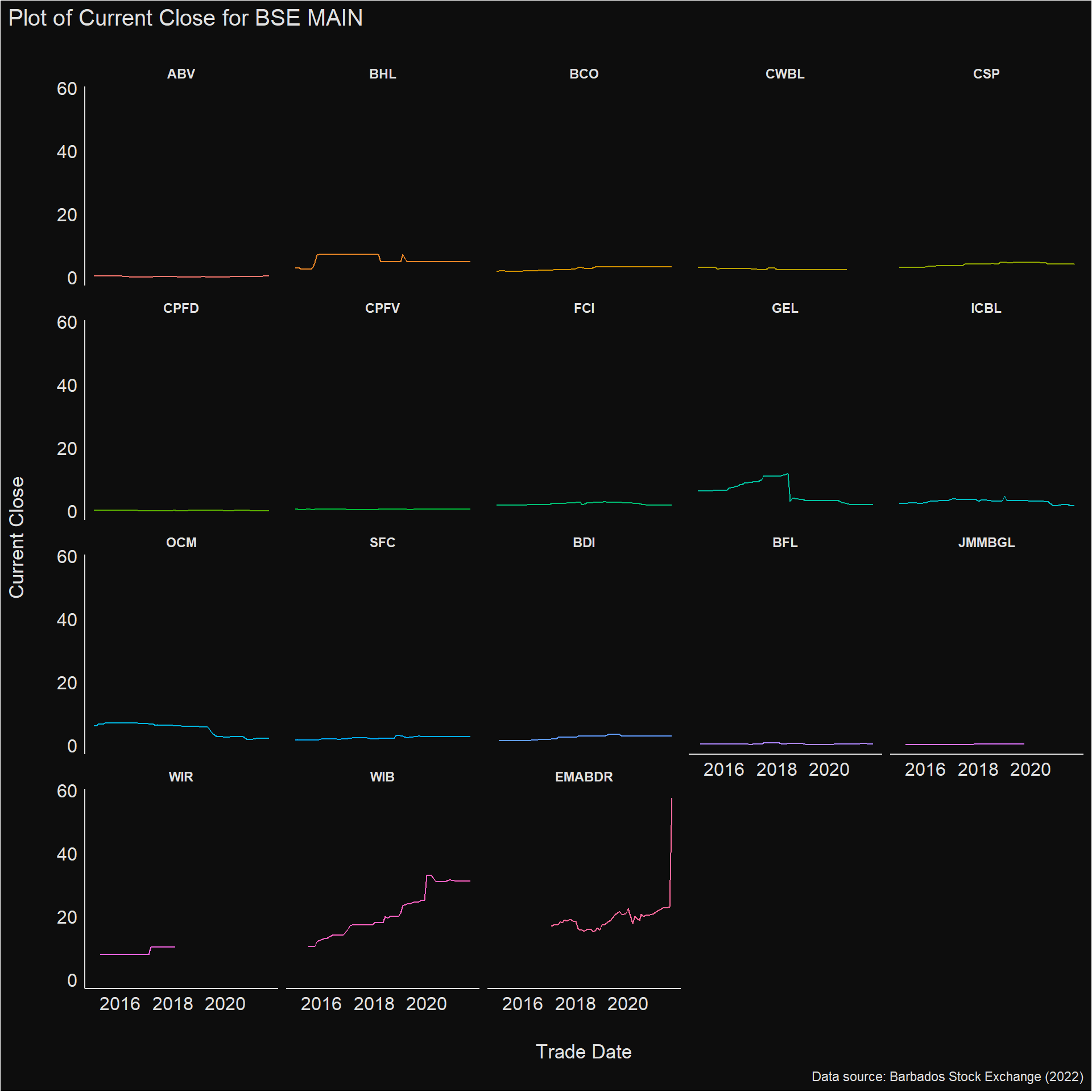
data_clean %>%
  filter(Title == "Fixed Income") %>%
  ggplot(aes(x = `Trade Date`,
             y = `Current Close`,
             colour = Security)) +
  geom_line(show.legend = FALSE) +
  facet_wrap(vars(Security)) +
  labs(title = "Plot of Current Close for BSE FIX",
       caption = "Data source: Barbados Stock Exchange (2022)") +
  see::theme_blackboard() +
  theme(axis.text.x = element_text(angle = 90)) +
  viridis::scale_fill_viridis()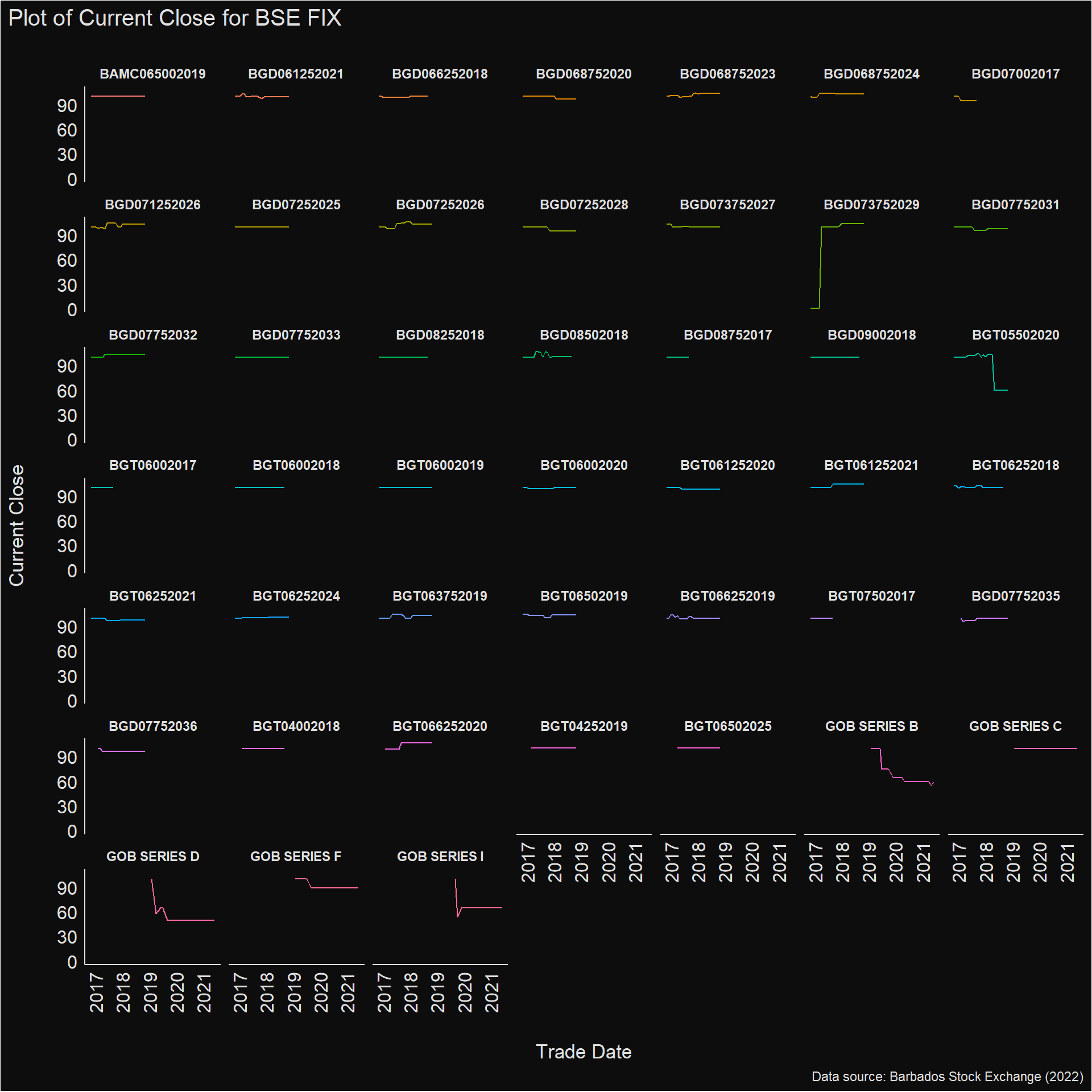
data_clean %>%
  filter(Title == "ISM") %>%
  ggplot(aes(x = `Trade Date`,
             y = `Current Close`,
             colour = Security)) +
  geom_line(show.legend = FALSE) +
  facet_wrap(vars(Security)) +
  labs(title = "Plot of Current Close for BSE ISM",
       caption = "Data source: Barbados Stock Exchange (2022)") +
  see::theme_blackboard() +
  viridis::scale_fill_viridis()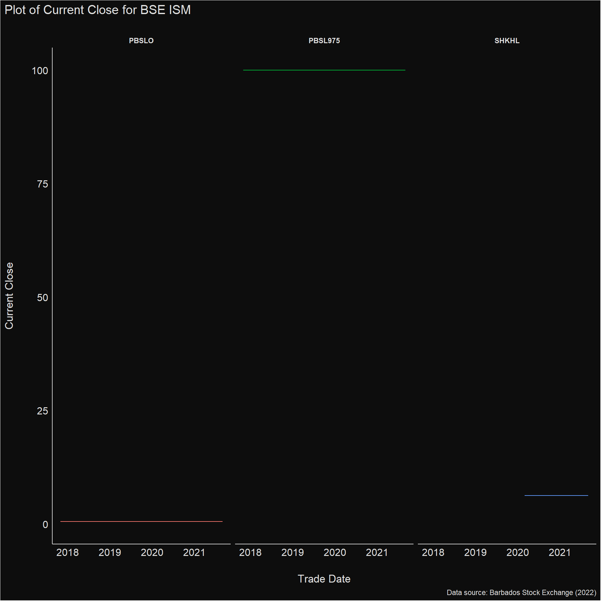
data_clean %>%
  filter(Title == "BSE ISM-BONDS") %>%
  ggplot(aes(x = `Trade Date`,
             y = `Current Close`,
             colour = Security)) +
  geom_line(show.legend = FALSE) +
  facet_wrap(vars(Security)) +
  labs(title = "Plot of Current Close for BSE ISM-BONDS",
       caption = "Data source: Barbados Stock Exchange (2022)") +
  see::theme_blackboard() +
  viridis::scale_fill_viridis()
This was a pretty interesting task.
If I revisit this, I’d like to confirm if BSE has an API of some form to use, and maybe I should learn a bit about stocks so I can do something interesting with the downloaded information.
Dario Clarke
Energy Analyst & Aspiring Data Analyst
My interests include sciences, religion and learning how people think.