A Dip into Weather

Last updated on 18 Jun 2021 R, Barbados

Image credit: Unsplash

The Intro

I hold a vested interest in the weather in Barbados. This isn’t just based on the ash fall we had received recently, but more due to working in the solar industry as an energy analyst.

I recently noticed on our meteorological services website a new section labelled Grafana which I naturally clicked. It led to me a dashboard that honestly blew me away. If I’m being completely honest, it’s not exactly what I expect from our government websites.

After some digging I came to the following conclusions:

This is a project powered by the 3D-PAWS (3D-Printed Automatic Weather Station) initiative
Barbados has at least one of the physical weather stations, but has integrated multiple pre-existing stations pushing data to the dashboard
The most important thing in my opinion; you can freely download data from this dashboard

There’s definitely interesting things you can find out about this project, for example these stations apparently use a raspberry pi for the brains. The project also 3D prints all the housings, connectors, and wire harnesses for the weather station and seems to have plans on making the designs to do so open source. I’m not sure how far they’ve gotten with it, but that’s pretty cool.

There’s a lot to dig into, but what I want to touch on here and now is the data itself I have access to.

The Data

The dashboard allows us to download data from their available stations. What we’ll be doing is downloading their irradiance information.

Now this setup supposedly has multiple ways to download data, but I seem to be currently limited to the old fashioned download from dashboard, so that’s exactly what I did.

I’ve manually downloaded the irradiance for each day going back a couple of days. The code will simply be made to handle either one or multiple files.

The Code

We’ll start by just loading our libraries.

library(tidyverse)

The Variables

These are the variables which will select the folder and files I wish to look at. In this way it should be easy to see I can easily change the code to read multiple file types, or variable with little hassle.

  file_type <- "csv"
  radiation_folder <- "radiation"
  radiation_data <- "grafana"

# Get possible files
files <- list.files(full.names = TRUE,
                    recursive = TRUE,
                    include.dirs = TRUE)

# Select Desired folder
used_file_radiation <- files[str_detect(files, radiation_folder)]
# Select Desired file
used_file_radiation <- files[str_detect(files, radiation_data)]
# Keep only the files which end with the given pattern
used_file_radiation <- used_file_radiation[str_detect(string = used_file_radiation,
                                                      pattern = paste0("(",file_type,")$"))]

# Download File(s) & transform
if(length(used_file_radiation) == 1){
  
  
  radiation_raw <- read_delim(used_file_radiation,
                              col_types = cols(Time = col_character(),
                                               Value = col_double()),
                              delim = ";",
                              na = "null") 
  
} else {
  
  radiation_raw <- used_file_radiation %>%
    map_df(~read_delim(.,
                       col_types = cols(Time = col_character(),
                                        Value = col_double()),
                       delim = ";",
                       na = "null")
    )
  
} 

radiation_raw <- radiation_raw %>%
  distinct() %>%
  # Split Datetime into Date and Time
  separate(col = Time,
           into = c("Date", "Time"),
           sep = "T") %>%
  # Discard Time Zone as it's not needed
  separate(col = Time,
           into = c("Time", NA),
           sep = "-") %>%
  # Convert date and time to correct format
  mutate(Date = lubridate::ymd(Date),
         Time =  hms::as_hms(Time),
         # Add back in Date - Time column in case it's useful
         Date_Time = lubridate::ymd_hms(paste0(Date,"T",Time)),
         Month = lubridate::month(Date, label = TRUE)
  ) %>%
  select(Series, Month, Date_Time, everything()) %>%
  arrange(Date_Time)

The Plot

Just to see that we’ve downloaded what we wanted, we can create a quick plot.

radiation_raw %>%
  filter(!is.na(Value)) %>%
  ggplot(aes( x = Date_Time, y = Value)) +
  geom_line(aes(colour = Series)) +
  facet_grid(Series~.,
             scales = "free_y") +
  labs(title = 'The Daily Irradiance',
       x = 'Time',
       y = 'Downwelling Irradiance (W/m^2)') +
  scale_y_continuous(labels = scales::comma) +
  theme(legend.position = "none")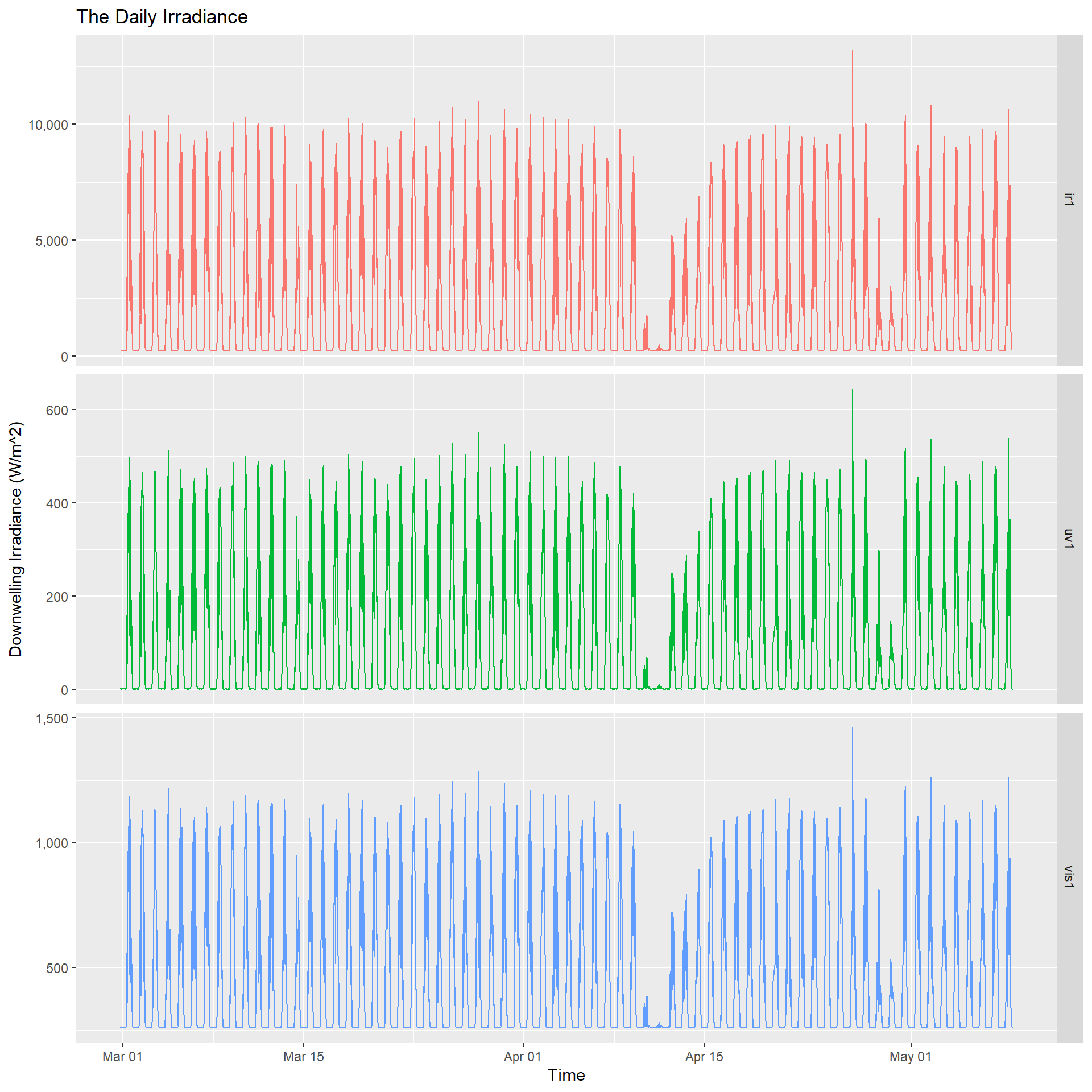

Well it does get what we want, but it looks a bit chaotic. Let’s instead plot the daily average for each month and see if that makes it easier to digest.

radiation_raw %>%
  filter(!is.na(Value)) %>%
  group_by(Month, Time, Series) %>%
  summarise(Radiation_mean = mean(Value),
            Radiation_sd = sd(Value)) %>%
  ungroup() %>%
  ggplot(aes(x = Time, y = Radiation_mean)) +
  geom_line(aes(colour = Series)) +
  geom_errorbar(aes(ymin = Radiation_mean - Radiation_sd,
                    ymax = Radiation_mean + Radiation_sd),
                width = 0.05,
                alpha = 0.3) +
  facet_grid(Series ~ Month,
             scales = "free_y") +
  labs(title = 'The Average Daily Irradiance',
       x = 'Time',
       y = 'Downwelling Irradiance (W/m^2)',
       subtitle = 'The mean daily irradiance per month',
       caption = 'includes standard deviation for each point') +
  scale_y_continuous(labels = scales::comma) +
  theme(axis.text.x = element_text(angle = 90),
        legend.position = "none")

## `summarise()` has grouped output by 'Month', 'Time'. You can override using the `.groups` argument.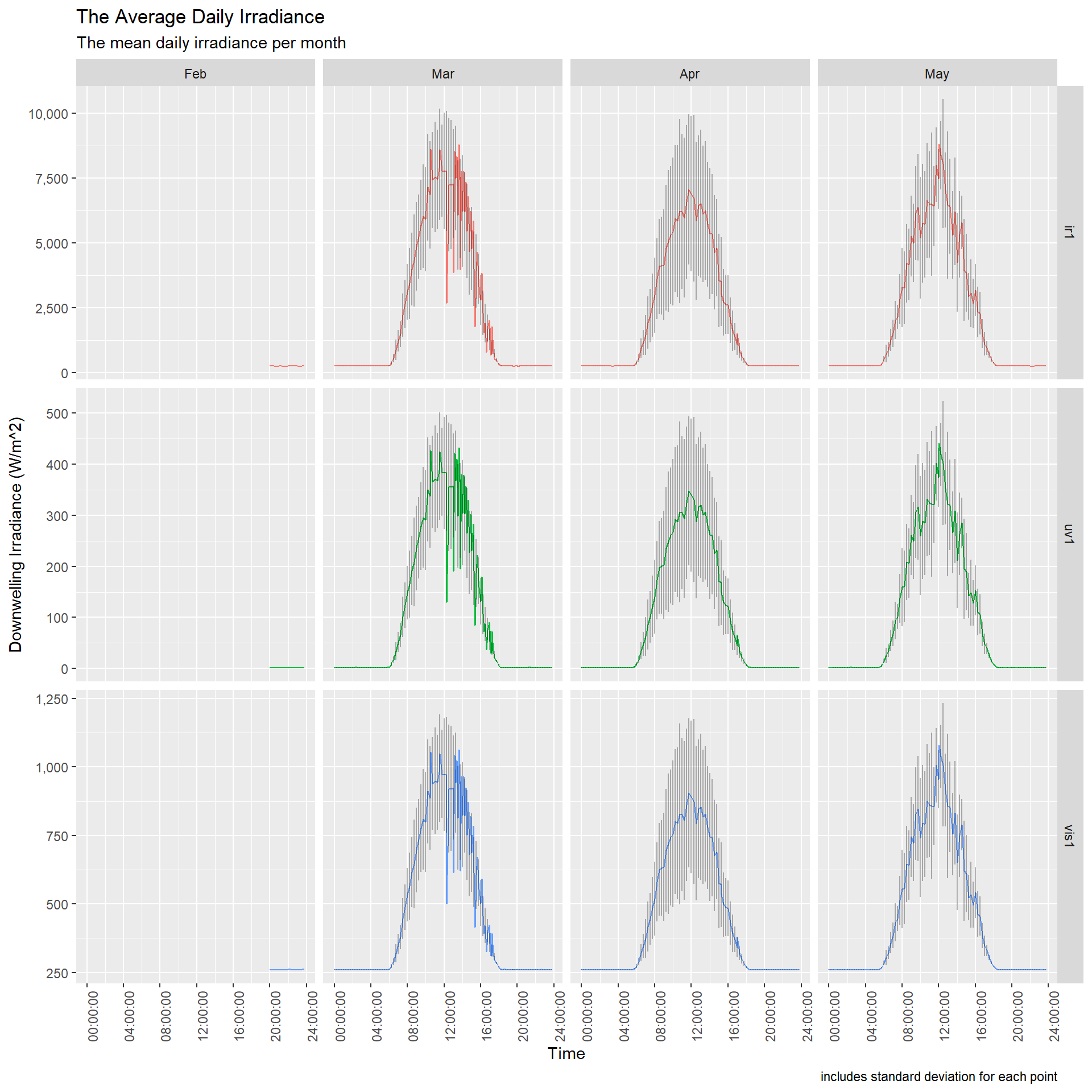

Hopefully I’ve shown how easy it is to use r to transform our data and visualise it.

It wouldn’t take much for me to create a template or a parametrised file to easily change inputs.

I also could easily feed this data into a solar model and use it to check for performance discrepancies due to weather.

I personally used Excel for all of this work before, and to be frank I can do it easily in that tool (I’ll never betray Excel 😀), but my experience with Excel and r are vastly different. I’ve only truly started using r recently while I’ve used Excel since university and straight through my entire career.

This should hopefully hint at how useful r can be in an energy analyst’s pipeline.

sessionInfo() %>%
  print(., locale = FALSE)

## R version 4.1.0 (2021-05-18)
## Platform: x86_64-w64-mingw32/x64 (64-bit)
## Running under: Windows 10 x64 (build 19043)
## 
## Matrix products: default
## 
## attached base packages:
## [1] stats     graphics  grDevices utils     datasets  methods   base     
## 
## other attached packages:
## [1] forcats_0.5.1   stringr_1.4.0   dplyr_1.0.6     purrr_0.3.4    
## [5] readr_1.4.0     tidyr_1.1.3     tibble_3.1.2    ggplot2_3.3.4  
## [9] tidyverse_1.3.1
## 
## loaded via a namespace (and not attached):
##  [1] tidyselect_1.1.1  xfun_0.24         bslib_0.2.5.1     haven_2.4.1      
##  [5] colorspace_2.0-1  vctrs_0.3.8       generics_0.1.0    htmltools_0.5.1.1
##  [9] yaml_2.2.1        utf8_1.2.1        rlang_0.4.11      jquerylib_0.1.4  
## [13] pillar_1.6.1      withr_2.4.2       glue_1.4.2        DBI_1.1.1        
## [17] dbplyr_2.1.1      modelr_0.1.8      readxl_1.3.1      lifecycle_1.0.0  
## [21] munsell_0.5.0     blogdown_1.3      gtable_0.3.0      cellranger_1.1.0 
## [25] rvest_1.0.0       evaluate_0.14     labeling_0.4.2    knitr_1.33       
## [29] fansi_0.5.0       highr_0.9         broom_0.7.7       Rcpp_1.0.6       
## [33] backports_1.2.1   scales_1.1.1      jsonlite_1.7.2    farver_2.1.0     
## [37] fs_1.5.0          hms_1.1.0         digest_0.6.27     stringi_1.6.2    
## [41] bookdown_0.22     grid_4.1.0        cli_2.5.0         tools_4.1.0      
## [45] magrittr_2.0.1    sass_0.4.0        crayon_1.4.1      pkgconfig_2.0.3  
## [49] ellipsis_0.3.2    xml2_1.3.2        reprex_2.0.0      lubridate_1.7.10 
## [53] rstudioapi_0.13   assertthat_0.2.1  rmarkdown_2.9     httr_1.4.2       
## [57] R6_2.5.0          compiler_4.1.0

Weather Solar