Harvesting Real Estate
 Image credit: Unsplash
The Intro
I find one of the strange road bumps you don’t expect in practicing data analytics is finding the data in the first place. Yes the world is currently overflowing with information, for instance the amount of data worldwide was estimated to be 44 zettabytes at the beginning of 2020, and we’re not slowing down. Now zetta is the prefix for 1 sextillion, or 21 zeroes behind the 1, that’s only 1 - 2 zeroes lower than the estimated number of stars in the universe.
Yet even with all of this data, the question remains, how pertinent is any of this information to me. I’m in Barbados, and the things I’m interested in definitely involve where I live, but looking for first hand data online for Barbados doesn’t return a great deal of results. It feels like an information desert, yet just like an oasis, the data can still be found.
One way is through web scraping, what this entails is collecting information, manually or otherwise, from a website or websites to be used.
The Preliminaries
Before we do any scraping, we need to do so ethically. Many websites have robots.txt which informs us on what scraping behaviour is allowed for the site. In our case, it would also be useful to read the terms and agreements to ensure web scraping is allowed. I’m included this since I found some sites whose robots.txt allows scraping but terms and conditions read in the contrary.
They are r packages (e.g. robotstxt) which allow you to check a site’s robots.txt in a r session, or websites (e.g. this one) which can be used to check as well. I chose to use the website in this case.
I recommend this website also for reading more about web scraping and robots.txt.
The site I found for this example is:
- Barbadian
- Allows for scraping in its robots.txt
- Its terms and conditions does not disallow scraping.
We’ll be moving forward with this site, but I wish to respect their privacy and will neither be indicating the name of the site nor showing any particular set of data which may be used to identify it, or any particular party or individual on their website.
The Data
The data we’ll be scraping is real estate information in Barbados.
The Code
We’ll start by just loading our libraries.
The main library of interest today is rvest which will be doing the brunt of the work for collecting information.
library(tidyverse)
library(rvest)
library(leaflet)
The Variables
We’ll be using a particular set of variables which I won’t be displaying here, sorry if that makes the code more difficult to understand.
# Please respect the privacy of the website
#
# This function calls identifiable variable of the website

if(!exists("hid_var", mode = "function")) {
  source("hid_var.R")
}
hid_var()
Web scraping with rvest involves:
- reading the entire page as html with
read_html
- If you view the page’s source, you will see the html code which this function will be reading. For Chrome & Edge you can currently do this by right clicking and selecting “view page source”.
- choosing the html tags & elements of interest with
html_elements
Within the html code are elements, usually denoted with some start and end tags
<...>…</...>.html_elementsallows us to select certain tags to collect their contents (the element) using CSS selectors, or XPath expressions.For my purpose, I used selector gadget to find the CSS selector I was interested in.
- choosing additional information of the html tags / elements in the form of attributes with
html_attr
- The attribute is found in the start tag and can be used to isolate additional details. In the example,
<a href="https://example.com">An Example Site</a>. The tag is<a>which has the attributehref.
They are other functions, but we’ll only be using these ones.
We will write our code to read multiple pages which will be implemented using a function to read each page.
We’ll open a connection to each page, read each page, and then close our connection to it on each iteration to ensure this works without hiccups.
We then combine the results from each page using map_dfr which will create one combined dataframe by appending each page’s results by row.
# Get the website Data


# Download property to find pages to scrape
temp_property_id <- map_dfr(1:row_limit, function(i) {

  # simple and effective progress indicator
  # cat(".")

  # download the page of interest
  pg <- paste0(page_begin,
               i,
               page_end) %>%
    url() %>%
    read_html()

  # close connection to the page of interest
  paste0(page_begin,
         i,
         page_end) %>%
    url() %>%
    close()

  # Check lengths of the three points of interest
  length_1 <- length(i)

  length_2 <- pg %>%
    html_elements(temp_1) %>%
    html_text() %>%
    length()

  length_3 <- pg %>%
    html_elements("a") %>%
    html_attr("onclick") %>%
    as_tibble() %>%
    filter(str_detect(string = value,
                      pattern = "LoadMap")) %>%
    as_vector() %>%
    length()

  # Select the max length between the three points of interest
  max_length <- max(c(length_1, length_2, length_3))

  # Place points of interest in a dataframe, and repeat a dummy value until they are the same length as the max length to avoid mismatched columns
  data.frame(
    web_page = c(i,
                 rep(i, max_length - length_1)),
    property_id = c(
      pg %>%
        html_elements(temp_1) %>%
        html_attr("onclick") %>%
        parse_number(),
      rep(i, max_length - length_2)),
    location = c(
      pg %>%
        html_elements("a") %>%
        html_attr("onclick") %>%
        as_tibble() %>%
        filter(str_detect(string = value,
                          pattern = "LoadMap")) %>%
        as_vector(),
      rep(i, max_length - length_3)),
    stringsAsFactors=FALSE)
})

# Display five random rows in generated dataframe
sample(x = 1:nrow(temp_property_id),
       size = 5,
       replace = FALSE) %>%
  temp_property_id[.,] %>%
  #obscure variable to use for identification
  mutate(property_id = "00000",
         location = paste( head(strsplit(location, '')[[1]], 14), collapse = "")
         ) %>%
  as_tibble() %>%
  gt::gt() %>%
  gt::tab_header(
    title = "Sample Values",
    subtitle = "Sample taken from initial scraped dataset"
)| Sample Values | ||
|---|---|---|
| Sample taken from initial scraped dataset | ||
| web_page | property_id | location |
| 168 | 00000 | LoadMap('13.16 |
| 28 | 00000 | LoadMap('13.16 |
| 374 | 00000 | LoadMap('13.16 |
| 183 | 00000 | LoadMap('13.16 |
| 262 | 00000 | LoadMap('13.16 |
We’ll clean this dataframe by isolating the latitude and longitude where possible, and doing a quick pass to remove coordinates which don’t fall in a certain distance around Barbados.
temp_property_id <- temp_property_id %>%
  separate(col = location,
           into = c("latitude", "longitude", NA),
           sep = ",") %>%
  # Simple sanity check for the values for latitude & longitude
  mutate(latitude = parse_number(latitude),
         latitude = if_else(latitude > 13.044347 & latitude < 13.335841,
                            latitude,
                            NA_real_),
         longitude = parse_number(longitude),
         longitude = if_else(longitude > -59.647765 & longitude < -59.410176,
                             longitude,
                             NA_real_))
## Warning: Expected 3 pieces. Additional pieces discarded in 5940 rows [1, 2, 3,
## 4, 5, 6, 7, 8, 9, 10, 11, 12, 13, 14, 15, 16, 17, 18, 19, 20, ...].## Warning: 1348 parsing failures.
## row col expected actual
## 3716 -- a number LoadMap(''
## 3717 -- a number LoadMap(''
## 3732 -- a number LoadMap(''
## 3733 -- a number LoadMap(''
## 3735 -- a number LoadMap(''
## .... ... ........ ..........
## See problems(...) for more details.## Warning: 1348 parsing failures.
## row col expected actual
## 3716 -- a number ''
## 3717 -- a number ''
## 3732 -- a number ''
## 3733 -- a number ''
## 3735 -- a number ''
## .... ... ........ ......
## See problems(...) for more details.# Display five random rows in generated dataframe
sample(x = 1:nrow(temp_property_id),
size = 5,
replace = FALSE) %>%
temp_property_id[.,] %>%
#obscure variable to use for identification
mutate(property_id = "00000",
latitude = round(latitude, 2),
longitude = round(longitude, 2)
) %>%
as_tibble() %>%
gt::gt() %>%
gt::tab_header(
title = "Sample Values",
subtitle = "Sample taken from initial scraped dataset"
)| Sample Values | |||
|---|---|---|---|
| Sample taken from initial scraped dataset | |||
| web_page | property_id | latitude | longitude |
| 98 | 00000 | 13.16 | -59.43 |
| 208 | 00000 | 13.14 | NA |
| 275 | 00000 | NA | NA |
| 242 | 00000 | 13.14 | -59.43 |
| 315 | 00000 | NA | NA |
We will use the property id to read each of the pages we’re interested in. On each page, our points of interest do not always appear, and when they do appear, they don’t always appear in the same order.
We will accommodate for this by ensuring our code will insert a ‘NA’ when the point of interest isn’t found and reorganising the collected data to properly group the information.
The only new function added is the use of html_text which allows us to take the text from an element.
if (!any( str_detect(list.files(full.names = TRUE,
                                recursive = TRUE,
                                include.dirs = TRUE),
                     "realestate.RData")
)
){

  raw_length <- nrow(temp_property_id)

  # Scrape the relevant details
  raw_data <- map_dfr(1:raw_length, function(i) {
    # simple but effective progress indicator
    cat(".")

    pg <- read_html(url(paste0(raw_page_begin,
                               temp_property_id$property_id[i],
                               raw_page_end)))

    close(url(paste0(raw_page_begin,
                     temp_property_id$property_id[i],
                     raw_page_end)))

    # the ifelse checks if the desired value exists, if yes, take the value, if no insert NA
    data.frame(
      row_1 = ifelse(
        length(html_text(html_elements(pg, type_1))) == 0,
        NA_character_,
        html_text(html_elements(pg, type_1))
      ),
      row_2 = ifelse(
        length(html_text(html_elements(pg, type_2))) == 0,
        NA_character_,
        html_text(html_elements(pg, type_2))
      ),
      row_3 = ifelse(
        length(html_text(html_elements(pg, type_3))) == 0,
        NA_character_,
        html_text(html_elements(pg, type_3))
      ),
      row_4 = ifelse(
        length(html_text(html_elements(pg, type_4))) == 0,
        NA_character_,
        html_text(html_elements(pg, type_4))
      ),
      row_5 = ifelse(
        length(html_text(html_elements(pg, type_5))) == 0,
        NA_character_,
        html_text(html_elements(pg, type_5))
      ),
      row_6 = ifelse(
        length(html_text(html_elements(pg, type_6))) == 0,
        NA_character_,
        html_text(html_elements(pg, type_6))
      ),
      row_7 = ifelse(
        length(html_text(html_elements(pg, type_7))) == 0,
        NA_character_,
        html_text(html_elements(pg, type_7))
      ),
      row_0 = ifelse(
        length(html_text(html_elements(pg,type_8))) == 0,
        NA_character_,
        html_text(html_elements(pg,type_8))
      ),
      title_1 = ifelse(
        length(html_text(html_elements(pg,type_9))) == 0,
        NA_character_,
        html_text(html_elements(pg,type_9))
      ),
      title_2 = ifelse(
        length(html_text(html_elements(pg,type_10))) == 0,
        NA_character_,
        html_text(html_elements(pg,type_10))
      ),
      title_3 = ifelse(
        length(html_text(html_elements(pg,type_11))) == 0,
        NA_character_,
        html_text(html_elements(pg,type_11))
      ),
      title_4 = ifelse(
        length(html_text(html_elements(pg,type_12))) == 0,
        NA_character_,
        html_text(html_elements(pg,type_12))
      ),
      title_5 = ifelse(
        length(html_text(html_elements(pg,type_13))) == 0,
        NA_character_,
        html_text(html_elements(pg,type_13))
      ),
      title_6 = ifelse(
        length(html_text(html_elements(pg,type_14))) == 0,
        NA_character_,
        html_text(html_elements(pg,type_14))
      ),
      title_7 = ifelse(
        length(html_text(html_elements(pg,type_15))) == 0,
        NA_character_,
        html_text(html_elements(pg,type_15))
      ),
      title_0 = ifelse(
        length(html_text(html_elements(pg,type_16))) == 0,
        NA_character_,
        html_text(html_elements(pg,type_16))
      ),
      description = ifelse(
        length(html_text(html_elements(pg,type_a))) == 0,
        NA_character_,
        html_text(html_elements(pg,type_a))
      ),
      realtor = ifelse(
        length(html_text(html_elements(pg,type_b))) == 0,
        NA_character_,
        html_text(html_elements(pg,type_b))
      ),
      blurb = ifelse(
        length(html_text(html_elements(pg,type_17))) == 0,
        NA_character_,
        # This uses `paste`, allowing us to combine multiple rows into one string
        paste(html_text(html_elements(pg,type_17)), collapse = " ")
      ),
      # We collected these values earlier, so we won't need to insert NA here
      latitude = temp_property_id$latitude[i],
      longitude = temp_property_id$longitude[i],
      link = paste0(raw_page_begin,
                    temp_property_id$property_id[i],
                    raw_page_end),
      stringsAsFactors=FALSE)

  })


  # Display five random rows in generated dataframe
  sample(x = 1:nrow(raw_data),
         size = 5,
         replace = FALSE) %>%
    raw_data[.,] %>%
  # remove variables which may identify locations
  select(!(description:link)) %>%
    as_tibble() %>%
    gt::gt() %>%
  gt::tab_header(
    title = "Sample Values",
    subtitle = "Sample taken from scraped dataset"
  )

}
We will clean this dataset by sorting the data into appropriate columns and pull some useful features from the collected unstructured text which we labelled blurb.
# Clean the Raw Data
# I currently like using case_when here because it's easy for me to read and I can easily edit as desired.
# If you use a more efficient method, let me know.

if (!any( str_detect(list.files(full.names = TRUE,
                                recursive = TRUE,
                                include.dirs = TRUE),
                     "realestate.RData")
)
){

  data <- raw_data %>%
    mutate(
      # Collect the price into one column
      price = case_when(
        title_0 == "Sale Price" ~ row_0,
        title_1 == "Sale Price" ~ row_1,
        title_2 == "Sale Price" ~ row_2,
        title_3 == "Sale Price" ~ row_3,
        title_4 == "Sale Price" ~ row_4,
        title_5 == "Sale Price" ~ row_5,
        title_6 == "Sale Price" ~ row_6,
        title_7 == "Sale Price" ~ row_7,
        TRUE                    ~ NA_character_
      ),
      # Collect the property status into one column
      property_status = case_when(
        title_0 == "Property Status" ~ row_0,
        title_1 == "Property Status" ~ row_1,
        title_2 == "Property Status" ~ row_2,
        title_3 == "Property Status" ~ row_3,
        title_4 == "Property Status" ~ row_4,
        title_5 == "Property Status" ~ row_5,
        title_6 == "Property Status" ~ row_6,
        title_7 == "Property Status" ~ row_7,
        TRUE                         ~ NA_character_
      ),
      # Collect the property type into one column
      property_type = case_when(
        title_0 == "Property Type" ~ row_0,
        title_1 == "Property Type" ~ row_1,
        title_2 == "Property Type" ~ row_2,
        title_3 == "Property Type" ~ row_3,
        title_4 == "Property Type" ~ row_4,
        title_5 == "Property Type" ~ row_5,
        title_6 == "Property Type" ~ row_6,
        title_7 == "Property Type" ~ row_7,
        TRUE                       ~ NA_character_
      ),
      # Collect the number of bedrooms into one column
      bedroom_no = case_when(
        title_0 == "Bedrooms" ~ row_0,
        title_1 == "Bedrooms" ~ row_1,
        title_2 == "Bedrooms" ~ row_2,
        title_3 == "Bedrooms" ~ row_3,
        title_4 == "Bedrooms" ~ row_4,
        title_5 == "Bedrooms" ~ row_5,
        title_6 == "Bedrooms" ~ row_6,
        title_7 == "Bedrooms" ~ row_7,
        TRUE                  ~ NA_character_
      ),
      # Collect the number of bathrooms into one column
      bathroom_no = case_when(
        title_0 == "Bathrooms" ~ row_0,
        title_1 == "Bathrooms" ~ row_1,
        title_2 == "Bathrooms" ~ row_2,
        title_3 == "Bathrooms" ~ row_3,
        title_4 == "Bathrooms" ~ row_4,
        title_5 == "Bathrooms" ~ row_5,
        title_6 == "Bathrooms" ~ row_6,
        title_7 == "Bathrooms" ~ row_7,
        TRUE                   ~ NA_character_
      ),
      # Collect the year built into one column
      year_built = case_when(
        title_0 == "Year Built" ~ row_0,
        title_1 == "Year Built" ~ row_1,
        title_2 == "Year Built" ~ row_2,
        title_3 == "Year Built" ~ row_3,
        title_4 == "Year Built" ~ row_4,
        title_5 == "Year Built" ~ row_5,
        title_6 == "Year Built" ~ row_6,
        title_7 == "Year Built" ~ row_7,
        TRUE                    ~ NA_character_
      ),
      # Collect the building area into one column
      bld_area = case_when(
        title_0 == "Building Area" ~ row_0,
        title_1 == "Building Area" ~ row_1,
        title_2 == "Building Area" ~ row_2,
        title_3 == "Building Area" ~ row_3,
        title_4 == "Building Area" ~ row_4,
        title_5 == "Building Area" ~ row_5,
        title_6 == "Building Area" ~ row_6,
        title_7 == "Building Area" ~ row_7,
        TRUE                       ~ NA_character_
      ),
      # Collect the property area into one column
      pty_area = case_when(
        title_0 == "Property Area" ~ row_0,
        title_1 == "Property Area" ~ row_1,
        title_2 == "Property Area" ~ row_2,
        title_3 == "Property Area" ~ row_3,
        title_4 == "Property Area" ~ row_4,
        title_5 == "Property Area" ~ row_5,
        title_6 == "Property Area" ~ row_6,
        title_7 == "Property Area" ~ row_7,
        TRUE                       ~ NA_character_
      ),
      # Create feature for beach access
      beach_access = case_when(
        str_detect(blurb, regex("Beach", ignore_case = T)) ~ TRUE,
        TRUE                                               ~ FALSE
      ),
      # Create feature for pool access
      pool_access = case_when(
        str_detect(blurb, regex("Pool", ignore_case = T)) ~ TRUE,
        TRUE                                              ~ FALSE
      ),
      # Create feature for golf access
      golf_access = case_when(
        str_detect(blurb, regex("Golf", ignore_case = T)) ~ TRUE,
        TRUE                                              ~ FALSE
      ),
      # Create feature for furnished building
      furnished = case_when(
        str_detect(blurb, regex("Furnish", ignore_case = T)) ~ TRUE,
        TRUE                                                 ~ FALSE
      ),
      # Create feature for currency used
      currency = case_when(
        str_detect(price,"(BB)") ~ "BBD",
        str_detect(price,"(US)") ~ "USD",
        TRUE ~ NA_character_),
      # Create feature for rent availability
      rent_available = case_when(
        str_detect(price,regex("\\s(rent)|^(rent)|\\s(lease)|^(lease)", ignore_case = T)) ~ TRUE,
        TRUE ~ FALSE),
      # Create feature for location by Parish
      parish = case_when(
        str_detect(description, "Christ Church") ~ "Christ Church",
        str_detect(description, "St. Andrew")    ~ "St. Andrew",
        str_detect(description, "St. George")    ~ "St. George",
        str_detect(description, "St. James")     ~ "St. James",
        str_detect(description, "St. John")      ~ "St. John",
        str_detect(description, "St. Joseph")    ~ "St. Joseph",
        str_detect(description, "St. Lucy")      ~ "St. Lucy",
        str_detect(description, "St. Michael")   ~ "St. Michael",
        str_detect(description, "St. Peter")     ~ "St. Peter",
        str_detect(description, "St. Philip")    ~ "St. Philip",
        str_detect(description, "St. Thomas")    ~ "St. Thomas",
        TRUE                                     ~ NA_character_
      ),
      # Parse the values which should be numbers
      price = parse_number(price),
      # Convert any number which was found as acres to sq. ft.
      pty_area = case_when(
        str_detect(pty_area,
                   regex("acre",
                         ignore_case = T)) ~ parse_number(pty_area) * 43560.04,
        str_detect(blurb,
                   regex("[:digit:](|\\.[:digit:])\\s+(acre)",
                         ignore_case = T)) ~  parse_number(
                           str_extract(blurb,
                                       regex("[:digit:](|\\.[:digit:])\\s+(acre)",
                                             ignore_case = T))
                         ) * 43560.04,
        TRUE ~ parse_number(pty_area)
      ),
      bld_area = parse_number(bld_area),
      bedroom_no = parse_number(bedroom_no),
      bathroom_no = parse_number(bathroom_no),
      year_built = parse_number(year_built),
      # Create the feature for price per square foot
      # We make some basic assumptions about what will likely be a price per square foot
      price_per_sqft = case_when(
        price < 100 ~ price,
        price > 100 & price < 5000 ~ NA_real_,
        price > 5000 & property_type == "Land" & !is.na(pty_area) ~ price / pty_area,
        price > 5000 & property_type == "Land" & !is.na(bld_area) ~ price / bld_area,
        price > 5000 & property_type != "Land" & !is.na(bld_area) ~ price / bld_area,
        price > 5000 & property_type != "Land" & !is.na(pty_area) ~ price / pty_area,
        TRUE ~ NA_real_
      ),
      # Remove any infinity values
      price_per_sqft = ifelse(is.infinite(price_per_sqft), NA_real_, price_per_sqft)
    ) %>%
    select(
      price,
      price_per_sqft,
      currency,
      property_status,
      property_type,
      rent_available,
      bedroom_no,
      bathroom_no,
      beach_access,
      pool_access,
      golf_access,
      furnished,
      bld_area,
      pty_area,
      year_built,
      realtor,
      latitude,
      longitude,
      parish,
      description,
      link
    )
  data <- na_if(data, "-")

} else{
  files <- list.files(full.names = TRUE,
                      recursive = TRUE,
                      include.dirs = TRUE)

  # Select Desired folder
  used_file <- files[str_detect(files, "realestate.RData")]

  load(used_file)

  rm(files,
     used_file)
}

# Display five random rows in generated dataframe
sample(x = 1:nrow(data),
       size = 5,
       replace = FALSE) %>%
  data[.,] %>%
  # remove variables which may identify locations
  select(!(realtor:link)) %>%
  as_tibble() %>%
  gt::gt() %>%
  gt::tab_header(
    title = "Sample Values",
    subtitle = "Sample taken from cleaned dataset"
  ) %>%
  gt::fmt_number(
    columns = c(price_per_sqft,
                bedroom_no,
                bathroom_no,
                bld_area,
                pty_area),
    decimals = 0,
    suffixing = TRUE
  ) %>%
  gt::fmt_currency(
    columns = price,
    suffixing = TRUE,
    currency = "BBD"
)| Sample Values | ||||||||||||||
|---|---|---|---|---|---|---|---|---|---|---|---|---|---|---|
| Sample taken from cleaned dataset | ||||||||||||||
| price | price_per_sqft | currency | property_status | property_type | rent_available | bedroom_no | bathroom_no | beach_access | pool_access | golf_access | furnished | bld_area | pty_area | year_built |
| $695.00K | 320 | BBD | Available | Apartment Block | FALSE | 6 | 4 | FALSE | FALSE | FALSE | TRUE | 2K | 6K | 2005 |
| $565.00K | 218 | BBD | Available | House | FALSE | 4 | 3 | FALSE | FALSE | FALSE | FALSE | 3K | NA | NA |
| $775.00K | 214 | BBD | Available | Other | FALSE | 5 | 5 | FALSE | FALSE | FALSE | FALSE | 4K | 20K | NA |
| $590.00K | 16 | BBD | Available | Land | FALSE | NA | NA | FALSE | FALSE | FALSE | FALSE | NA | 36K | NA |
| $80.59K | 16 | BBD | Sold | Land | FALSE | NA | NA | FALSE | FALSE | FALSE | FALSE | NA | 5K | NA |
We’ll save our dataframe for use at a later date.
# Save file
if (!any( str_detect(list.files(full.names = TRUE,
                                recursive = TRUE,
                                include.dirs = TRUE),
                     "realestate.RData")
)
) { save(data, file = "realestate.RData")
}
The Statistics
With this we’re finished with our web scraping and can pursue exploring and better cleaning our data if choose to.
Before I close this post, let’s take a quick look at what we did scrape by generating a summary table with pricing in Barbados.
data %>%
  group_by(property_type) %>%
  summarise(amount = n(),
            `price (mean)` = mean(price),
            `price (standard deviation)` = sd(price),
            `price sq.ft (mean)` = mean(price_per_sqft, na.rm = TRUE),
            `price sq.ft (standard deviation)` = sd(price_per_sqft, na.rm = TRUE)) %>%
  arrange(`price sq.ft (mean)`) %>%
  rename(`property type` = property_type) %>%
  ungroup() %>%
  gt::gt() %>%
  gt::tab_header(
    title = "Summary Statistics"
  ) %>%
  gt::fmt_number(
    columns = amount,
    decimals = 0,
    suffixing = TRUE
  ) %>%
  gt::fmt_currency(
    columns = c(`price (mean)`,
                `price (standard deviation)`,
                `price sq.ft (mean)`,
                `price sq.ft (standard deviation)`),
    suffixing = TRUE,
    currency = "BBD"
)| Summary Statistics | |||||
|---|---|---|---|---|---|
| property type | amount | price (mean) | price (standard deviation) | price sq.ft (mean) | price sq.ft (standard deviation) |
| Land | 3K | $766.06K | $2.98M | $24.12 | $43.07 |
| Unfinished Structure | 24 | $278.33K | $183.16K | $88.29 | $60.54 |
| Commercial Property - No Building | 24 | $1.32M | $1.24M | $114.63 | $221.41 |
| Warehouse | 21 | $3.62M | $4.27M | $170.10 | $137.61 |
| Commercial Property with Building/s | 86 | $3.01M | $4.04M | $227.91 | $167.17 |
| Hotel | 25 | $9.33M | $8.16M | $230.04 | $183.01 |
| Chattel House | 1 | $250.00K | NA | $292.91 | NA |
| Plantation House | 37 | $6.18M | $9.88M | $313.55 | $477.18 |
| Apartment Block | 102 | $1.47M | $1.70M | $355.44 | $745.34 |
| Shop | 12 | $2.26M | $2.43M | $368.87 | $263.76 |
| House | 2K | $1.66M | $3.48M | $391.57 | $849.17 |
| Other | 35 | $3.07M | $4.46M | $409.09 | $382.13 |
| Guest House | 6 | $2.03M | $701.19K | $452.81 | $458.53 |
| Town House | 384 | $1.13M | $886.38K | $528.38 | $304.17 |
| Restaurant | 17 | $2.30M | $2.36M | $557.24 | $488.67 |
| Office | 43 | $2.93M | $3.45M | $603.71 | $1.42K |
| Apartment / Condo | 612 | $1.25M | $1.45M | $751.04 | $404.75 |
| 12-month BWS Rental property | 4 | $2.02M | $1.66M | $1.06K | $582.31 |
| Bank-owned property | 4 | $2.81M | $4.66M | $1.22K | $2.33K |
| NA | 14 | NA | NA | NaN | NA |
We see there are 20 property types, but with the amount of cleaning we’ve done so far, examining the category for Land seems to be the most useful. It has the lowest deviation.
We’ll drill in on the specific summary statistics for Land, divided by Parish.
data %>%
  filter(property_type == "Land") %>%
  ggplot(aes(x = parish, y = log(price_per_sqft))) +
  geom_boxplot(aes(fill = parish)) +
labs(title = 'The Log Price ($/sq.ft.) for Land in Barbados',
       x = 'Parish',
       y = 'Log Price',
       caption = 'please remember these are log values and are more useful for comparing orders of magnitude') +
  scale_y_continuous(labels = scales::dollar_format(prefix = "log($",
                                                    suffix = "/sq.ft.)")) +
  theme(axis.text.x = element_text(angle = 90),
        legend.position = "none")
## Warning: Removed 180 rows containing non-finite values (stat_boxplot).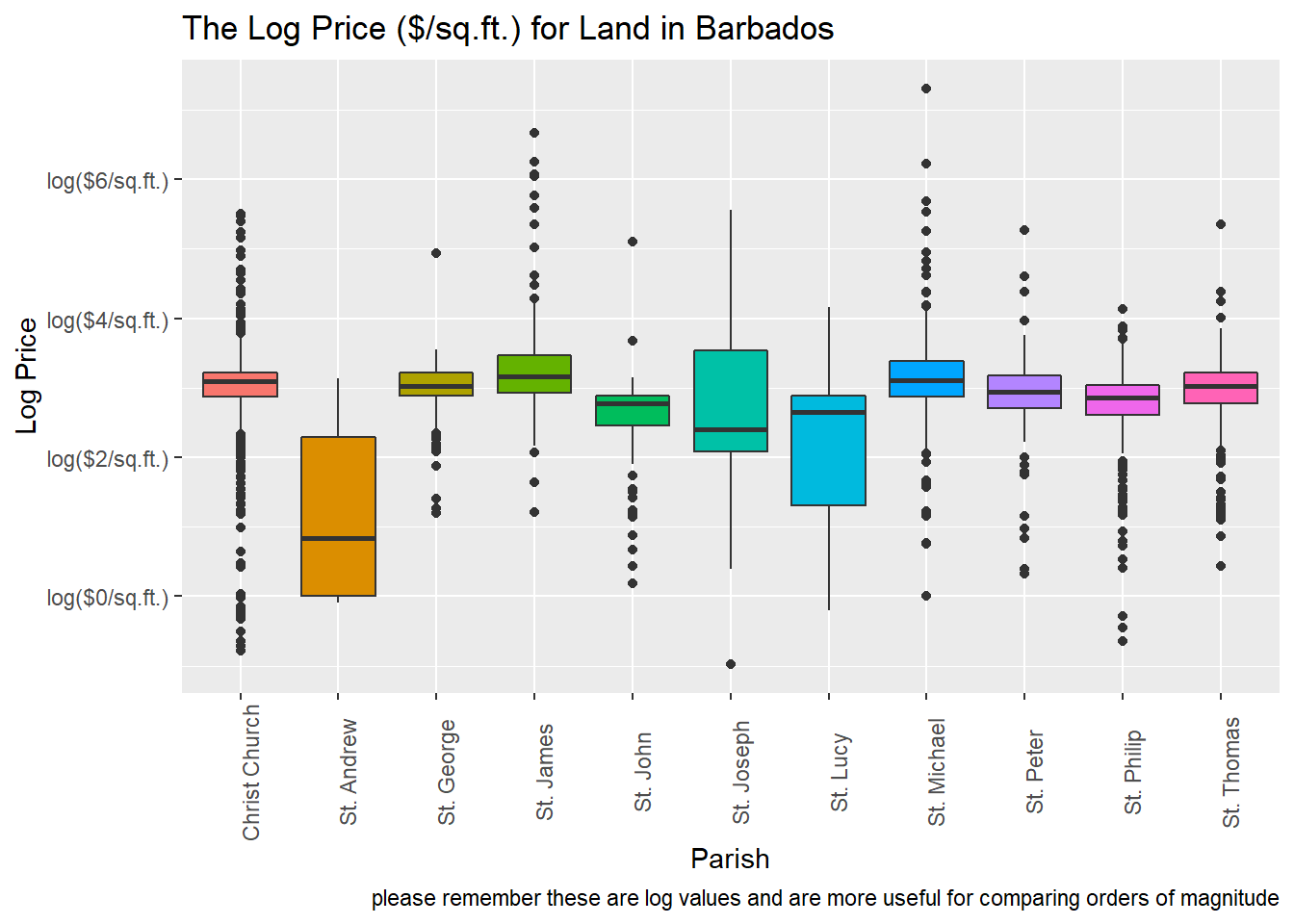
The above plot shows us that for certain parishes (see St. Michael, St. Joseph and St. James) they are large outliers in the $/sq.ft in terms of how expensive they are. St. Andrew and St. Lucy also seem to tend in the opposite direction and are cheaper than other parishes. Overall there’s quite a bit of variance in the price of land in general.
data %>%
  filter(property_type == "Land") %>%
  group_by(property_type, parish) %>%
  summarise(amount = n(),
            `price (mean)` = mean(price),
            `price (standard deviation)` = sd(price),
            `price sq.ft (mean)` = mean(price_per_sqft, na.rm = TRUE),
            `price sq.ft (standard deviation)` = sd(price_per_sqft, na.rm = TRUE)) %>%
  arrange(`price sq.ft (mean)`) %>%
  rename(`property type` = property_type) %>%
  ungroup() %>%
  ggplot(aes(x = parish, y = `price sq.ft (mean)`)) +
  geom_col(aes(fill = parish)) +
  geom_errorbar(aes(ymin = `price sq.ft (mean)` - `price sq.ft (standard deviation)`,
                    ymax = `price sq.ft (mean)` + `price sq.ft (standard deviation)`),
                width = 0.5,
                alpha = 0.8) +
labs(title = 'The Average Price ($/sq.ft.) for Land in Barbados',
       x = 'Parish',
       y = 'Average Price ($/sq.ft.)',
       caption = 'includes standard deviation for each point') +
  scale_y_continuous(labels = scales::dollar_format(suffix = "/sq.ft.")) +
  theme(axis.text.x = element_text(angle = 90),
        legend.position = "none")
## `summarise()` has grouped output by 'property_type'. You can override using the `.groups` argument.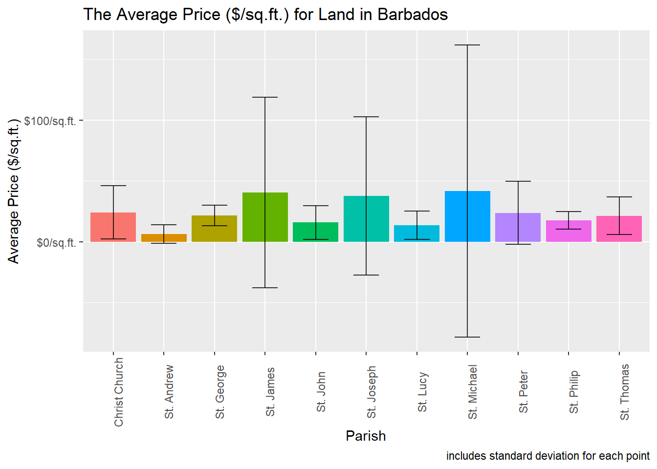
What we mentioned about high outliers seems to be true as we see our error bars for certain values literally goes into the negative range which shows the influence of outliers in that group and also suggests that the average for those particular bars are also skewed.
We’ll simply put these values in a table for you to make your own conclusion.
data %>%
  filter(property_type == "Land") %>%
  group_by(property_type, parish) %>%
  summarise(amount = n(),
            `price (mean)` = mean(price),
            `price (standard deviation)` = sd(price),
            `price sq.ft (mean)` = mean(price_per_sqft, na.rm = TRUE),
            `price sq.ft (standard deviation)` = sd(price_per_sqft, na.rm = TRUE)) %>%
  arrange(`price sq.ft (mean)`) %>%
  rename(`property type` = property_type) %>%
  ungroup() %>%
  gt::gt() %>%
  gt::tab_header(
    title = "Summary Statistics"
  ) %>%
  gt::fmt_number(
    columns = amount,
    decimals = 0,
    suffixing = TRUE
  ) %>%
  gt::fmt_currency(
    columns = c(`price (mean)`,
                `price (standard deviation)`,
                `price sq.ft (mean)`,
                `price sq.ft (standard deviation)`),
    suffixing = TRUE,
    currency = "BBD"
  )
## `summarise()` has grouped output by 'property_type'. You can override using the `.groups` argument.| Summary Statistics | ||||||
|---|---|---|---|---|---|---|
| property type | parish | amount | price (mean) | price (standard deviation) | price sq.ft (mean) | price sq.ft (standard deviation) |
| Land | St. Andrew | 9 | $955.78K | $1.66M | $6.27 | $7.80 |
| Land | St. Lucy | 44 | $1.28M | $4.79M | $13.57 | $11.52 |
| Land | St. John | 156 | $275.74K | $1.01M | $15.82 | $13.96 |
| Land | St. Philip | 604 | $551.61K | $2.88M | $17.57 | $7.13 |
| Land | St. Thomas | 284 | $569.78K | $1.16M | $21.29 | $15.51 |
| Land | St. George | 345 | $360.98K | $1.62M | $21.53 | $8.58 |
| Land | St. Peter | 132 | $1.50M | $5.48M | $23.68 | $25.83 |
| Land | Christ Church | 711 | $603.46K | $1.96M | $24.04 | $21.87 |
| Land | St. Joseph | 35 | $1.26M | $3.74M | $37.66 | $65.16 |
| Land | St. James | 234 | $1.40M | $4.06M | $40.35 | $78.35 |
| Land | St. Michael | 190 | $1.98M | $5.30M | $41.76 | $120.22 |
Lastly we can generate a map showing the locations for each point which shows the location, price per sq.ft. and property type.
data %>%
  filter( !is.na(price_per_sqft) ) %>%
  mutate(pop = paste0(property_type,": ","$",round(price_per_sqft,2))
           ) %>%
  leaflet() %>%
  addTiles() %>%
  addMarkers(
    lat = ~latitude,
    lng = ~longitude,
    label = ~property_type,
    popup = ~pop,
    clusterOptions = markerClusterOptions()
    ) #%>%
#widgetframe::frameWidget(.,width = "100%")The Conclusion
From this exercise we see an example of web scraping in r, along with handling a non-standard website.
We also can see that this type of information still has its flaws, for example look at the map and you can still find points in the ocean, and from manual checks I found other input errors for different locations. Taking from a primary source does not negate the need for cleaning.
I should also point out that this information is still only useful as a proxy, for example the prices listed are from the real estate agents, these prices won’t necessarily be the final price paid and thus may not be what property actually costs in Barbados.
In a future post, we may revisit this data for exploration and to see what statistics are used when dealing with real estate.
sessionInfo() %>%
  print(., locale = FALSE)
## R version 4.1.0 (2021-05-18)
## Platform: x86_64-w64-mingw32/x64 (64-bit)
## Running under: Windows 10 x64 (build 19043)
##
## Matrix products: default
##
## attached base packages:
## [1] stats graphics grDevices utils datasets methods base
##
## other attached packages:
## [1] leaflet_2.0.4.1 rvest_1.0.0 forcats_0.5.1 stringr_1.4.0
## [5] dplyr_1.0.6 purrr_0.3.4 readr_1.4.0 tidyr_1.1.3
## [9] tibble_3.1.2 ggplot2_3.3.3 tidyverse_1.3.1
##
## loaded via a namespace (and not attached):
## [1] Rcpp_1.0.6 lubridate_1.7.10 assertthat_0.2.1 digest_0.6.27
## [5] utf8_1.2.1 R6_2.5.0 cellranger_1.1.0 backports_1.2.1
## [9] reprex_2.0.0 evaluate_0.14 highr_0.9 httr_1.4.2
## [13] blogdown_1.3 pillar_1.6.1 rlang_0.4.11 readxl_1.3.1
## [17] rstudioapi_0.13 jquerylib_0.1.4 checkmate_2.0.0 rmarkdown_2.8
## [21] labeling_0.4.2 selectr_0.4-2 htmlwidgets_1.5.3 munsell_0.5.0
## [25] broom_0.7.6 compiler_4.1.0 modelr_0.1.8 xfun_0.23
## [29] pkgconfig_2.0.3 htmltools_0.5.1.1 tidyselect_1.1.1 bookdown_0.22
## [33] fansi_0.5.0 crayon_1.4.1 dbplyr_2.1.1 withr_2.4.2
## [37] grid_4.1.0 jsonlite_1.7.2 gtable_0.3.0 lifecycle_1.0.0
## [41] DBI_1.1.1 magrittr_2.0.1 scales_1.1.1 cli_2.5.0
## [45] stringi_1.6.2 farver_2.1.0 fs_1.5.0 xml2_1.3.2
## [49] bslib_0.2.5.1 ellipsis_0.3.2 generics_0.1.0 vctrs_0.3.8
## [53] tools_4.1.0 glue_1.4.2 hms_1.1.0 crosstalk_1.1.1
## [57] yaml_2.2.1 colorspace_2.0-1 gt_0.3.0 knitr_1.33
## [61] haven_2.4.1 sass_0.4.0Dario Clarke
Energy Analyst & Aspiring Data Analyst
My interests include sciences, religion and learning how people think.